An alert says an observation is unusual under a reference model. It does not say which component changed, whether the reference model remains suitable, or whether an automatic adjustment will help. Drift detection becomes useful when the alert leads to a bounded investigation and a defensible decision about which observations still describe the current system.
A stopping interval and a monitoring limit answer different questions. The lab's seven-look interval estimates one stable run's observed Bell score. A monitor compares successive batches with a reference state. Reusing cumulative science counts as though they were independent monitor batches confuses those roles and can hide a new change inside a large historical average.
Build a monitor with visible assumptions
The teaching fixture uses separate batches with 1,000 shots in each of three bases. For its known baseline model, p=0.02 and q=0.01, the analytic mean score is 0.955894. The batch standard deviation is approximately 0.00462651. Three-standard-deviation monitoring limits are therefore approximately 0.942014 and 0.969774.
These are known-model control limits, not 95% confidence bounds for an unknown mean and not a product specification. A chart fitted from finite calibration data has additional estimation uncertainty. Its behavior also depends on the distribution and dependence of the monitored observations. NIST's control-chart discussion.
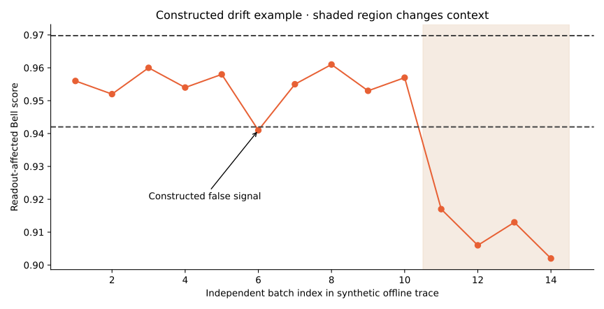
The displayed series is an explicitly constructed offline trace. Rows 1–10 retain the teaching baseline, with row 6 chosen as an illustrative false signal. Rows 11–14 represent an injected change to p=0.08 while q remains 0.01. They are not randomly captured hardware or Aer observations, and they do not measure detection power.
| Batch | Favorable parity outcomes across all bases | Score | Known teaching context |
|---|---|---|---|
| 5 | 2,916 | 0.958 | baseline |
| 6 | 2,882 | 0.941 | baseline; illustrative false signal |
| 7 | 2,910 | 0.955 | baseline |
| 10 | 2,914 | 0.957 | baseline |
| 11 | 2,834 | 0.917 | injected change |
| 12 | 2,812 | 0.906 | injected change |
| 13 | 2,826 | 0.913 | injected change |
| 14 | 2,804 | 0.902 | injected change |
“Favorable” means even parity in XX/ZZ and odd parity in YY. With total favorable count K, the score is K/2,000−0.5. The changed model's analytic mean is 0.912676, explaining the direction of the later values. An operator observing these numbers would not know the injected cause; that information belongs to the teaching scenario.
False alarms are part of the operating design
Under independent normal observations with known parameters, two-sided three-sigma limits signal about 0.27% of the time. Repeating such checks makes an eventual false alarm unsurprising. For this particular Bell monitor, the exact discrete binomial calculation instead gives approximately 0.0031042 per check, or 0.31042%. Matching a mean and variance does not make the underlying distribution exactly normal.
A signal can justify immediate investigation without proving a changed process. Check measurement integrity, the acquisition context, recent software and calibration changes, and whether the signal repeats under a planned follow-up. Recurrence is not automatically independent confirmation: adjacent observations may share environmental disturbances or overlapping data.
The teaching fixture includes a separate analytic correlation example. A stationary Gaussian sequence with lag-k correlation 0.8^k has variance inflation of 8.6 for a mean of 100 observations. Its effective sample size for that mean is approximately 11.63. An independence-based three-sigma limit for the mean would then signal about 30.63% of the time. This calculation concerns averages and joint dependence; it does not say correlation changes every individual observation's marginal distribution. NIST on autocorrelated monitoring.
Preserve the boundary between diagnosis and recovery
The lab also has a different artifact: a captured Aer drift scenario using p=0.02 and degraded readout q=0.16. It rejects at 200 shots per basis. Its separate recovery run restores q=0.01 under a new context identifier and accepts at 5,000. Do not confuse that capture with the constructed p=0.08 monitor trace above.
Recovery should collect evidence about the new state. Pooling old degraded data into its interval estimates a mixture of histories, not necessarily the restored operating condition. Keep the old run, its rejection, and the recovery relationship. If an operational policy pauses after the first alert, later plotted points must be labeled as an offline illustration or a documented investigation and resumption.
Exercise and worked answer
Calculate the scores for K=2,882 and K=2,834. Which crosses the lower monitoring limit? Does the first prove drift? If an engineer averages 100 correlated residuals from the analytic example, how much is the naive standard error understated?
Worked answer: The scores are 0.941 and 0.917; both are below 0.942014. In the constructed ground truth, the first is a false signal and the second follows an injected change. Observations alone do not reveal that distinction. With variance inflation 8.6, the correct standard error of the mean is √8.6≈2.93 times the independence-based value. Investigate the signal and dependence before interpreting a narrow interval or taking an irreversible control action. Telemetry, SLOs, and Service Error Budgets explains how these alerts relate to a service promise.